install.packages(c("pins", "arrow", "sf", "duckdb", "DBI"))![]()
Introduction
WECA’s shared data platform provides 18 curated datasets covering local authority lookups, greenhouse gas emissions, energy performance certificates, deprivation indices, postcode centroids, tenure, and spatial boundaries. All data is stored on Amazon S3 and accessible through two complementary routes:
- Pins (R or Python): Read datasets directly into data frames. Best for quick exploratory analysis, filtering, and visualisation.
- DuckLake (SQL via DuckDB CLI): Query datasets with SQL, join across tables, use pre-built WECA-filtered views, and browse the data catalogue. Best for complex queries and when you need to work across multiple tables.
Both routes read from the same underlying data. Choose whichever fits your workflow – or use both.
TipThe 10-minute promise
If you follow the Prerequisites section below, you will be able to read your first dataset within 10 minutes.
This guide covers everything you need: package installation, AWS credential setup, reading data via pins, querying the DuckLake catalogue with SQL, working with spatial data, and troubleshooting common issues. Python equivalents are provided in Appendix A.
Prerequisites and Setup
Before accessing data, you need three things: R packages, the DuckDB command-line tool (for SQL access), and AWS credentials. This section walks through each.
R Packages
Install the core packages. This guide assumes you already have the tidyverse installed.
| Package | Purpose |
|---|---|
pins |
Connect to the S3 board, list/read/download datasets |
arrow |
Read parquet files (required for large and spatial datasets) |
sf |
Handle spatial data (GeoParquet to sf objects) |
duckdb |
DuckDB database driver for R (used for local queries) |
DBI |
Database interface (works with duckdb) |
DuckDB Installation
The DuckDB command-line interface (CLI) is required for querying the DuckLake catalogue. The R duckdb package (v1.4.4) does not include the ducklake extension, so SQL queries against the catalogue must be run through the CLI.
- Download the DuckDB CLI from https://duckdb.org/docs/installation/.
- Place the
duckdbexecutable somewhere on your PATH. - Verify installation:
duckdb --versionv1.4.4 (Andium) 6ddac802ff
Note
The DuckDB CLI is only needed for DuckLake SQL queries (Section 5). For reading data via pins, you only need the R packages above.
AWS Credentials
You need AWS credentials to access the shared S3 bucket (stevecrawshaw-bucket). Request an access key ID and secret access key from the data owner (distributed via Keeper).
Step 1: Create the credentials file
Create the file at:
- Windows:
C:\Users\USERNAME\.aws\credentials - Linux/Mac:
~/.aws/credentials
If the .aws directory does not exist, create it first. Paste the following content, replacing the placeholders with your actual keys - get these from Steve:
[default]
aws_access_key_id = <YOUR_ACCESS_KEY_ID>
aws_secret_access_key = <YOUR_SECRET_ACCESS_KEY>
Step 2: Create the config file
Create the file at:
- Windows:
C:\Users\USERNAME\.aws\config - Linux/Mac:
~/.aws/config
Paste the following content:
[default]
region = eu-west-2
output = json
WarningRegion must be eu-west-2
The S3 bucket is in the eu-west-2 (London) region. Using any other region will cause “Access Denied” errors or 301 redirects. Always set region = eu-west-2.
Step 3: Verify access
Pick whichever tool you use day-to-day. A successful result from any one method confirms your credentials are working.
R (pins):
library(pins)
board <- board_s3(bucket = "stevecrawshaw-bucket",
                  prefix = "pins/",
                   region = "eu-west-2")
pin_list(board)
DuckDB CLI:
INSTALL aws; LOAD aws;
CREATE OR REPLACE SECRET (
    TYPE s3, PROVIDER credential_chain,
    CHAIN config, REGION 'eu-west-2'
);
SELECT * FROM glob('s3://stevecrawshaw-bucket/*');
AWS CLI (optional):
aws s3 ls s3://stevecrawshaw-bucket/
TipTroubleshooting credentials
If you get “Access Denied” or “No credentials” errors, see the Troubleshooting section. Common causes: wrong region, missing profile name [default], or a .txt extension accidentally added by your text editor.
Available Datasets
The platform provides 18 base tables and 12 pre-built views. The table below is a quick reference; for full column-level details, query the datasets_catalogue and columns_catalogue programmatically (see Querying the Data Catalogue).
Base Tables
| Name | Description | Spatial | Approx. Rows |
|---|---|---|---|
bdline_ua_lep_diss_tbl |
Boundary line UA LEP dissolved | Yes | 1 |
bdline_ua_lep_tbl |
Boundary line UA LEP | Yes | 5 |
bdline_ua_weca_diss_tbl |
Boundary line UA WECA dissolved | Yes | 1 |
bdline_ward_lep_tbl |
Boundary line wards LEP | Yes | 70 |
boundary_lookup_tbl |
Boundary lookup (LA/ward/LSOA codes) | – | 700 |
ca_boundaries_bgc_tbl |
Combined authority boundaries (BGC) | Yes | 11 |
ca_la_lookup_tbl |
Combined authority to local authority lookup | – | 106 |
codepoint_open_lep_tbl |
Codepoint Open postcodes LEP | Yes | 49,000 |
eng_lsoa_imd_tbl |
English LSOA Index of Multiple Deprivation | – | 33,000 |
iod2025_tbl |
Index of Deprivation 2025 | – | 33,000 |
la_ghg_emissions_tbl |
Local authority greenhouse gas emissions | – | 27,000 |
la_ghg_emissions_wide_tbl |
LA GHG emissions (wide format) | – | 6,000 |
lsoa_2021_lep_tbl |
LSOA 2021 boundaries (LEP area) | Yes | 700 |
open_uprn_lep_tbl |
Open UPRN addresses (LEP area) | Yes | 700,000 |
postcode_centroids_tbl |
Postcode centroids (all England) | – | 1,800,000 |
raw_domestic_epc_certificates_tbl |
Domestic EPC certificates (raw) | – | 19,000,000 |
raw_non_domestic_epc_certificates_tbl |
Non-domestic EPC certificates (raw) | – | 900,000 |
uk_lsoa_tenure_tbl |
UK LSOA tenure (Census 2021) | – | 35,000 |
Views (WECA-filtered)
The catalogue includes 12 views. Four are source views that reshape or join data; the remaining eight pre-filter data to the four WECA local authorities (Bath and North East Somerset, Bristol, North Somerset, South Gloucestershire). Views have names ending in _weca_vw, _vw, or _ods_vw.
| Name | Description |
|---|---|
ca_la_lookup_inc_ns_vw |
CA/LA lookup including North Somerset |
weca_lep_la_vw |
WECA LEP local authorities (4 rows) |
ca_la_ghg_emissions_sub_sector_ods_vw |
GHG emissions joined with CA/LA lookup |
epc_domestic_vw |
Domestic EPC with derived fields (construction year, tenure) |
la_ghg_emissions_weca_vw |
GHG emissions filtered to WECA LAs |
la_ghg_emissions_wide_weca_vw |
GHG emissions (wide) filtered to WECA LAs |
raw_domestic_epc_weca_vw |
Domestic EPC filtered to WECA LAs |
raw_non_domestic_epc_weca_vw |
Non-domestic EPC filtered to WECA LAs |
boundary_lookup_weca_vw |
Boundary lookup filtered to WECA LAs |
postcode_centroids_weca_vw |
Postcode centroids filtered to WECA LAs |
iod2025_weca_vw |
Index of Deprivation 2025 filtered to WECA LAs |
ca_la_lookup_weca_vw |
CA/LA lookup filtered to WECA LAs |
Note
Row counts are approximate. For exact current counts, query datasets_catalogue in DuckLake (see Section 5.5).
Accessing Data via Pins
The pins package is the primary way to read data from the platform into R. All datasets are stored as versioned parquet files on S3.
Creating a Board
Connect to the S3 board. You only need to do this once per session.
library(pins)

board <- board_s3(
  bucket = "stevecrawshaw-bucket",
  prefix = "pins/",
  region = "eu-west-2",
  versioned = TRUE
)
The versioned = TRUE parameter means you can access previous versions of datasets if needed.
Listing Datasets
See all available datasets on the board:
pin_list(board) [1] "bdline_ua_lep_diss_tbl"
[2] "bdline_ua_lep_tbl"
[3] "bdline_ua_weca_diss_tbl"
[4] "bdline_ward_lep_tbl"
[5] "boundary_lookup_tbl"
[6] "ca_boundaries_bgc_tbl"
[7] "ca_la_lookup_tbl"
[8] "codepoint_open_lep_tbl"
[9] "columns_catalogue"
[10] "datasets_catalogue"
[11] "eng_lsoa_imd_tbl"
[12] "iod2025_tbl"
[13] "la_ghg_emissions_tbl"
[14] "la_ghg_emissions_wide_tbl"
[15] "lsoa_2021_lep_tbl"
[16] "open_uprn_lep_tbl"
[17] "postcode_centroids_tbl"
[18] "raw_domestic_epc_certificates_tbl"
[19] "raw_non_domestic_epc_certificates_tbl"
[20] "uk_lsoa_tenure_tbl" Reading a Dataset
Read a dataset directly into an R data frame with pin_read(). Start with ca_la_lookup_tbl – it is small (106 rows) and loads instantly.
df <- pin_read(board, "ca_la_lookup_tbl")
head(df)
# A data frame: 6 × 5
LAD25CD LAD25NM CAUTH25CD CAUTH25NM ObjectId
* <chr> <chr> <chr> <chr> <dbl>
1 E08000001 Bolton E47000001 Greater Manchester 1
2 E08000002 Bury E47000001 Greater Manchester 2
3 E08000003 Manchester E47000001 Greater Manchester 3
4 E08000004 Oldham E47000001 Greater Manchester 4
5 E08000005 Rochdale E47000001 Greater Manchester 5
6 E08000006 Salford E47000001 Greater Manchester 6str(df)Classes 'tbl' and 'data.frame': 106 obs. of 5 variables:
$ LAD25CD : chr "E08000001" "E08000002" "E08000003" "E08000004" ...
$ LAD25NM : chr "Bolton" "Bury" "Manchester" "Oldham" ...
$ CAUTH25CD: chr "E47000001" "E47000001" "E47000001" "E47000001" ...
$ CAUTH25NM: chr "Greater Manchester" "Greater Manchester" "Greater Manchester" "Greater Manchester" ...
$ ObjectId : num 1 2 3 4 5 6 7 8 9 10 ...Accessing Metadata
Every dataset carries metadata including a description and column-level documentation:
meta <- pin_meta(board, "ca_la_lookup_tbl")
meta$title
[1] "Combined authority local authority boundaries"meta$user$columns$LAD25CD
[1] "Local authority district code 2025"
$LAD25NM
[1] "Local authority district name 2025"
$CAUTH25CD
[1] "Combined authority code 2025"
$CAUTH25NM
[1] "Combined authority name 2025"
$ObjectId
[1] "Objectid"Column descriptions come from the data catalogue and are embedded in each pin’s metadata. Use meta$user$column_types to see the data types.
Large Datasets
The raw_domestic_epc_certificates_tbl dataset contains approximately 19 million rows and is stored as a multi-file pin (multiple parquet files). For this table, pin_read() may be slow or fail. Use arrow::open_dataset() instead:
library(arrow)

# Download the parquet files
paths <- pin_download(board, "raw_domestic_epc_certificates_tbl")

# Open as an Arrow dataset (lazy -- does not load into memory)
ds <- open_dataset(paths)

# Query efficiently with dplyr
library(dplyr)
bristol_epcs <- ds |>
  filter(local_authority == "Bristol, City of") |>
  select(address1, current_energy_rating, potential_energy_rating) |>
  collect()
Tip
For any dataset, you can use pin_download() followed by arrow::read_parquet() if you prefer working with Arrow tables directly. This is also the required approach for spatial datasets (see Section 6).
Querying the DuckLake Catalogue
DuckLake provides SQL access to the same datasets. This is useful when you need to join tables, run aggregate queries, use pre-built WECA views, or browse the data catalogue. All DuckLake SQL runs through the DuckDB CLI (not the R duckdb package).
Installing Extensions
Open the DuckDB CLI and install the required extensions. This only needs to be done once – extensions are cached locally.
INSTALL ducklake;
LOAD ducklake;

INSTALL httpfs;
LOAD httpfs;

INSTALL aws;
LOAD aws;
For spatial queries, also install:
INSTALL spatial;
LOAD spatial;
Attaching the Catalogue
Each time you open a DuckDB CLI session, you need to create an S3 credential and attach the catalogue.
-- Create S3 credential (uses your ~/.aws/credentials file)
CREATE SECRET (TYPE s3, REGION 'eu-west-2', PROVIDER credential_chain);

-- Attach the DuckLake catalogue
ATTACH 'ducklake:data/mca_env.ducklake' AS lake
  (READ_ONLY, DATA_PATH 's3://stevecrawshaw-bucket/ducklake/data/');
ImportantYou need the .ducklake file locally
The file data/mca_env.ducklake is a small metadata file that must be on your local machine. Clone the repository to get it:
git clone <repo-url>
cd ducklake
The .ducklake file is only metadata (a few KB). The actual data lives on S3 and is fetched transparently when you run queries.
To see all available tables and views:
USE lake;
SHOW TABLES;
Basic SQL Queries
Select all rows from a small table:
SELECT * FROM lake.ca_la_lookup_tbl LIMIT 5;Filter with WHERE:
SELECT LAD25NM, population
FROM lake.ca_la_lookup_tbl
WHERE CAUTH25NM = 'West of England'
ORDER BY population DESC;
Aggregate with GROUP BY:
SELECT territorial_emissions_sector,
       ROUND(SUM(territorial_emissions_kt_co2e), 1) AS total_kt
FROM lake.la_ghg_emissions_tbl
WHERE local_authority_name IN ('Bristol, City of', 'Bath and North East Somerset',
                                'North Somerset', 'South Gloucestershire')
  AND year = 2021
GROUP BY territorial_emissions_sector
ORDER BY total_kt DESC;
Join tables:
SELECT l.LAD25NM, g.year,
       ROUND(SUM(g.territorial_emissions_kt_co2e), 1) AS total_emissions
FROM lake.la_ghg_emissions_tbl g
JOIN lake.ca_la_lookup_tbl l ON g.local_authority_code = l.LAD25CD
WHERE l.CAUTH25NM = 'West of England'
GROUP BY l.LAD25NM, g.year
ORDER BY g.year DESC, total_emissions DESC
LIMIT 8;
Using Views
WECA-filtered views pre-filter data to the four WECA local authorities, saving you from writing the same WHERE clause repeatedly.
-- Instead of filtering manually:
SELECT * FROM lake.la_ghg_emissions_tbl
WHERE local_authority_code IN ('E06000022','E06000023','E06000024','E06000025');

-- Use the WECA view directly:
SELECT * FROM lake.la_ghg_emissions_weca_vw;
-- List distinct authorities in a WECA view
SELECT DISTINCT local_authority_code, local_authority_name
FROM lake.la_ghg_emissions_weca_vw;Querying the Data Catalogue
The catalogue includes two metadata tables that describe every dataset and column programmatically.
List all datasets with descriptions and row counts:
SELECT name, description, type, row_count
FROM lake.datasets_catalogue
ORDER BY type, name;
Explore columns for a specific table:
SELECT column_name, data_type, description, example_1
FROM lake.columns_catalogue
WHERE table_name = 'la_ghg_emissions_tbl'
ORDER BY column_name;
Find spatial datasets:
SELECT name, geometry_type, crs, row_count
FROM lake.datasets_catalogue
WHERE geometry_type IS NOT NULL;
Time Travel
DuckLake keeps snapshots of your data. You can query a table as it existed at a previous version:
-- Query the table at version 1
SELECT COUNT(*) FROM lake.ca_la_lookup_tbl AT (VERSION => 1);

-- List available snapshots
SELECT * FROM lake.snapshots() ORDER BY snapshot_id DESC LIMIT 5;
Snapshots are retained for 90 days and then automatically cleaned up. Time travel is useful for auditing changes or recovering from accidental modifications.
Working with Spatial Data
Eight of the 18 datasets contain geometry columns and are stored as GeoParquet files on S3. These cover boundaries (UA, ward, LSOA), postcodes (Codepoint Open), addresses (UPRN), and combined authority areas.
WarningDo not use sfarrow
The sfarrow package fails on GeoParquet files produced by DuckDB because DuckDB does not write CRS metadata into the GeoParquet geo key. Always use the arrow + sf approach described below.
Reading GeoParquet Pins
Spatial pins must be read with pin_download() followed by arrow::read_parquet(), not with pin_read():
# Download the GeoParquet file
pin_path <- pin_download(board, "bdline_ua_lep_tbl")

# Read with arrow
arrow_tbl <- arrow::read_parquet(pin_path, as_data_frame = FALSE)
Converting to sf Objects
Convert the Arrow table to an sf object in two steps:
sf_obj <- sf::st_as_sf(as.data.frame(arrow_tbl))The two-step process (as.data.frame() then st_as_sf()) is needed because sf expects a data frame with a geometry column, and Arrow tables need explicit conversion.
sf_objSimple feature collection with 4 features and 3 fields
Geometry type: MULTIPOLYGON
Dimension: XY
Bounding box: xmin: 322292.8 ymin: 152770 xmax: 382605.5 ymax: 198319.9
CRS: NA
name code id shape
1 Bath and North East Somerset E06000022 1 MULTIPOLYGON (((376262.8 17...
2 City of Bristol E06000023 2 MULTIPOLYGON (((353416.3 18...
3 South Gloucestershire E06000025 3 MULTIPOLYGON (((364881.8 19...
4 North Somerset E06000024 4 MULTIPOLYGON (((349585 1781...Setting CRS
Notice that the CRS shows as NA above. DuckDB does not embed CRS metadata into GeoParquet files, so you must set it explicitly after reading.
sf_obj <- sf::st_set_crs(sf_obj, 27700)Most spatial tables use EPSG:27700 (British National Grid). The one exception is ca_boundaries_bgc_tbl, which uses EPSG:4326 (WGS84 latitude/longitude).
| Dataset | CRS |
|---|---|
bdline_ua_lep_diss_tbl |
EPSG:27700 |
bdline_ua_lep_tbl |
EPSG:27700 |
bdline_ua_weca_diss_tbl |
EPSG:27700 |
bdline_ward_lep_tbl |
EPSG:27700 |
ca_boundaries_bgc_tbl |
EPSG:4326 |
codepoint_open_lep_tbl |
EPSG:27700 |
lsoa_2021_lep_tbl |
EPSG:27700 |
open_uprn_lep_tbl |
EPSG:27700 |
You can also check the correct CRS from the pin metadata:
meta <- pin_meta(board, "bdline_ua_lep_tbl")
meta$user$crs
[1] "EPSG:27700"Plotting a Quick Map
Once the CRS is set, you can plot directly:
plot(sf_obj["name"])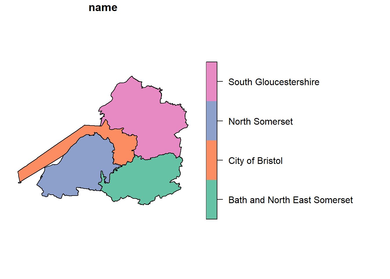
For a more polished map using ggplot2:
ggplot(sf_obj) +
  geom_sf(aes(fill = name), colour = "white") +
  theme_minimal() +
  labs(title = "WECA LEP Local Authorities",
       fill = "Authority") +
  theme(legend.position = "bottom")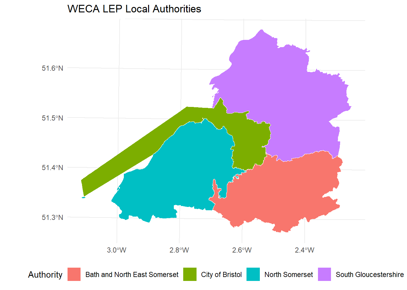
Troubleshooting
“Access Denied” or region errors
Symptom: S3 operations fail with “Access Denied”, 403, or 301 redirect errors.
Cause: The region is not set to eu-west-2, or credentials are missing/expired.
Fix:
- Check
~/.aws/configcontainsregion = eu-west-2. - In DuckDB, always specify
REGION 'eu-west-2'in the secret definition. - Verify your credentials have not expired – contact the data owner for new keys if needed.
“File not found” when attaching DuckLake
Symptom: ATTACH 'ducklake:data/mca_env.ducklake' fails with a file-not-found error.
Cause: The .ducklake catalogue file must be on your local machine. It is not hosted on S3.
Fix: Clone the repository and run DuckDB from the project root directory:
git clone <repo-url>
cd ducklake
duckdb
CRS shows as NA or OGC:CRS84
Symptom: After reading a spatial dataset, sf::st_crs() returns NA, or geopandas shows OGC:CRS84.
Cause: DuckDB does not embed CRS metadata into GeoParquet files.
Fix: Set the CRS explicitly after reading. Most tables use EPSG:27700; ca_boundaries_bgc_tbl uses EPSG:4326. See the CRS table above.
sfarrow fails on GeoParquet
Symptom: sfarrow::st_read_parquet() throws an error about missing CRS or geo key.
Cause: sfarrow requires full GeoParquet metadata including CRS, which DuckDB does not write.
Fix: Use arrow::read_parquet() followed by sf::st_as_sf() instead. Do not use sfarrow with these files.
Python board_s3 path format
Symptom: Python board_s3() fails with connection errors or “bucket not found”.
Cause: Python pins uses a different path format from R.
Fix: Use board_s3("stevecrawshaw-bucket/pins", versioned=True) – the bucket and prefix are combined in a single string. Do not pass them as separate parameters.
Python pin_read fails on EPC table
Symptom: board.pin_read("raw_domestic_epc_certificates_tbl") throws an error in Python.
Cause: The EPC table is a multi-file pin (exported in chunks). The Python pins library cannot handle multi-file pins with pin_read.
Fix: Use pyarrow directly:
import pyarrow.dataset as ds
paths = board.pin_download("raw_domestic_epc_certificates_tbl")
dataset = ds.dataset(paths, format="parquet")
df = dataset.to_table().to_pandas()
DuckLake extension not available in R
Symptom: dbExecute(con, "INSTALL ducklake") fails from the R duckdb package.
Cause: The R duckdb package (v1.4.4) does not include the ducklake extension.
Fix: Use the DuckDB CLI for all DuckLake queries. For data frame access, use pins instead – you do not need DuckLake for reading data into R.
Support and Contact
NoteUpdate before distributing
Replace the placeholders below with your team’s actual contact details before sharing this guide.
- Contact: Steve Crawshaw
- Repository: Report issues or request new datasets via the project GitHub repository.
- AWS access requests: Contact the Steve to receive credentials.
For urgent data access issues, check the Troubleshooting section first.
Appendix A: Python Equivalents
This appendix provides Python equivalents of the key R examples above. Python is a secondary access path – R is the primary supported language.
Pins Access
ImportantPython path format differs from R
In Python, board_s3() takes a single string "bucket/prefix" rather than separate bucket and prefix parameters. Note the absence of a trailing slash.
import os
os.environ.setdefault("AWS_DEFAULT_REGION", "eu-west-2")

from pins import board_s3

# Create board -- note the "bucket/prefix" format (no trailing slash)
board = board_s3("stevecrawshaw-bucket/pins", versioned=True)

# List datasets
board.pin_list()
# Read a dataset
df = board.pin_read("ca_la_lookup_tbl")
print(df.head())# Read metadata
meta = board.pin_meta("ca_la_lookup_tbl")
print(meta.title)
print(meta.user["columns"])
Warning
pin_read() fails on multi-file pins (e.g., the EPC table). Use pyarrow.dataset as shown in the Troubleshooting section.
DuckLake Queries
You can run DuckLake SQL from Python using the duckdb package:
import duckdb

conn = duckdb.connect()

# Install and load extensions
conn.execute("INSTALL ducklake; LOAD ducklake;")
conn.execute("INSTALL httpfs; LOAD httpfs;")
conn.execute("INSTALL aws; LOAD aws;")

# Create S3 credential
conn.execute("CREATE SECRET (TYPE s3, REGION 'eu-west-2', PROVIDER credential_chain);")

# Attach the DuckLake catalogue
conn.execute("""
    ATTACH 'ducklake:data/mca_env.ducklake' AS lake
    (READ_ONLY, DATA_PATH 's3://stevecrawshaw-bucket/ducklake/data/');
""")

# Query
df = conn.execute("SELECT * FROM lake.ca_la_lookup_tbl LIMIT 5").fetchdf()
print(df)
Note
Unlike R, the Python duckdb package does support the ducklake extension. You can run DuckLake queries directly from Python without the CLI.
Spatial Data with geopandas
import os
os.environ.setdefault("AWS_DEFAULT_REGION", "eu-west-2")

from pins import board_s3
import geopandas as gpd

board = board_s3("stevecrawshaw-bucket/pins", versioned=True)

# Download and read GeoParquet
path = board.pin_download("bdline_ua_lep_tbl")
gdf = gpd.read_parquet(path[0])

# CRS may show as OGC:CRS84 -- override to the correct CRS
gdf = gdf.set_crs("EPSG:27700", allow_override=True)

# Quick plot
gdf.plot(column="name", legend=True)
Warning
geopandas may report the CRS as OGC:CRS84 when GeoParquet lacks CRS metadata. Always use set_crs() with allow_override=True to set the correct CRS.
Appendix B: SQL Quick Reference
A brief SQL primer for analysts who are familiar with R but new to SQL. All examples use DuckLake tables.
SELECT – choose columns:
SELECT LAD25NM, population
FROM lake.ca_la_lookup_tbl;
R equivalent: df |> select(LAD25NM, population)
WHERE – filter rows:
SELECT LAD25NM, population
FROM lake.ca_la_lookup_tbl
WHERE CAUTH25NM = 'West of England';
R equivalent: df |> filter(CAUTH25NM == "West of England")
ORDER BY – sort results:
SELECT LAD25NM, population
FROM lake.ca_la_lookup_tbl
ORDER BY population DESC;
R equivalent: df |> arrange(desc(population))
LIMIT – return a fixed number of rows:
SELECT * FROM lake.la_ghg_emissions_tbl LIMIT 10;R equivalent: df |> head(10) or df |> slice_head(n = 10)
GROUP BY – aggregate:
SELECT CAUTH25NM, COUNT(*) AS n_las, SUM(population) AS total_pop
FROM lake.ca_la_lookup_tbl
GROUP BY CAUTH25NM
ORDER BY total_pop DESC;
R equivalent: df |> group_by(CAUTH25NM) |> summarise(n_las = n(), total_pop = sum(population))
JOIN – combine tables:
SELECT l.LAD25NM, g.year, g.territorial_emissions_kt_co2e
FROM lake.la_ghg_emissions_tbl g
JOIN lake.ca_la_lookup_tbl l
  ON g.local_authority_code = l.LAD25CD
WHERE l.CAUTH25NM = 'West of England'
  AND g.year = 2021;
R equivalent: left_join(ghg, lookup, by = c("local_authority_code" = "LAD25CD"))
Common aggregate functions:
| SQL | R equivalent | Description |
|---|---|---|
COUNT(*) |
n() |
Number of rows |
SUM(col) |
sum(col) |
Total |
AVG(col) |
mean(col) |
Average |
MIN(col) |
min(col) |
Minimum |
MAX(col) |
max(col) |
Maximum |
ROUND(col, 2) |
round(col, 2) |
Round to N decimals |